Tutorial part 3
In part 1 and part 2 we have learnt about portfolio lines. These are timeseries, or collections of timeseries, describing the volumes and/or prices during various delivery periods.
In this part, we’ll combine portfolio lines into a “portfolio state” (PfState) object. As we’ll see, some of the methods and properties we know from the PfLine class also apply here.
Example data
Let’s again use the mock functions to get some portfolio lines. (The parameter details here are not important, we just want some more-or-less realistic data). To change things up a bit from the previous tutorial parts, we’ll look at about 80 days in the autumn of 2024, in quarterhourly ("15min") resolution. And let’s localize the data to a specific timezone:
[1]:
import portfolyo as pf
import pandas as pd

index = pd.date_range(
    "2024-09-20", "2024-12-10", freq="15min", inclusive="left", tz="Europe/Berlin"
)
# Creating offtake portfolio line.
ts_offtake = -1 * pf.dev.w_offtake(index, avg=50)
offtake = pf.PfLine({"w": ts_offtake})
# Creating portfolio line with market prices (here: price-forward curve).
ts_prices = pf.dev.p_marketprices(index, avg=200)
prices = pf.PfLine({"p": ts_prices})

# Creating portfolio line with sourced volume.
ts_sourced_power1, ts_sourced_price1 = pf.dev.wp_sourced(
    ts_offtake, "QS", 0.3, p_avg=120
)
sourced_quarters = pf.PfLine({"w": ts_sourced_power1, "p": ts_sourced_price1})
ts_sourced_power2, ts_sourced_price2 = pf.dev.wp_sourced(
    ts_offtake, "MS", 0.2, p_avg=150
)
sourced_months = pf.PfLine({"w": ts_sourced_power2, "p": ts_sourced_price2})
sourced = pf.PfLine(
    {"quarter_products": sourced_quarters, "month_products": sourced_months}
)
We can now use these portfolio lines to create a portfolio state.
Portfolio State
The PfState class is used to hold information about offtake, market prices, and sourcing. Let’s create one from the portfolio lines we just created:
[2]:
pfs = pf.PfState(offtake, prices, sourced)

pfs
[2]:
PfState object.
. Start: 2024-09-20 00:00:00+02:00 (incl)    . Timezone    : Europe/Berlin
. End  : 2024-12-10 00:00:00+01:00 (excl)    . Start-of-day: 00:00:00
. Freq : <15 * Minutes> (7780 datapoints)
                                                w           q           p             r
                                               MW         MWh     Eur/MWh           Eur
──────── offtake
           2024-09-20 00:00:00 +0200        -45.8         -11
           2024-09-20 00:15:00 +0200        -44.4         -11
           ..                                  ..          ..          ..            ..
           2024-12-09 23:30:00 +0100        -60.5         -15
           2024-12-09 23:45:00 +0100        -58.3         -15
─●────── pnl_cost
 │         2024-09-20 00:00:00 +0200         45.8          11      136.54         1 564
 │         2024-09-20 00:15:00 +0200         44.4          11      135.21         1 500
 │         ..                                  ..          ..          ..            ..
 │         2024-12-09 23:30:00 +0100         60.5          15      167.89         2 540
 │         2024-12-09 23:45:00 +0100         58.3          15      167.21         2 436
 ├●───── sourced
 ││        2024-09-20 00:00:00 +0200         31.3           8      135.03         1 058
 ││        2024-09-20 00:15:00 +0200         31.3           8      135.03         1 058
 ││        ..                                  ..          ..          ..            ..
 ││        2024-12-09 23:30:00 +0100         35.7           9      126.09         1 124
 ││        2024-12-09 23:45:00 +0100         35.7           9      126.09         1 124
 │├───── quarter_products
 ││        2024-09-20 00:00:00 +0200         16.4           4      102.48           421
 ││        2024-09-20 00:15:00 +0200         16.4           4      102.48           421
 ││        ..                                  ..          ..          ..            ..
 ││        2024-12-09 23:30:00 +0100         13.4           3      111.14           372
 ││        2024-12-09 23:45:00 +0100         13.4           3      111.14           372
 │└───── month_products
 │         2024-09-20 00:00:00 +0200         14.9           4      170.85           637
 │         2024-09-20 00:15:00 +0200         14.9           4      170.85           637
 │         ..                                  ..          ..          ..            ..
 │         2024-12-09 23:30:00 +0100         22.3           6      135.07           752
 │         2024-12-09 23:45:00 +0100         22.3           6      135.07           752
 └────── unsourced
           2024-09-20 00:00:00 +0200         14.5           4      139.81           506
           2024-09-20 00:15:00 +0200         13.0           3      135.64           442
           ..                                  ..          ..          ..            ..
           2024-12-09 23:30:00 +0100         24.8           6      227.88         1 416
           2024-12-09 23:45:00 +0100         22.6           6      232.05         1 312
Note from how these portfolio lines were created, that offtake has negative values. The sign conventions are discussed here.
This portfolio state contains values for every quarterhour in the specified time period. Let’s see what features this class has, starting with two methods we already met when discussing the PfLine class.
Plotting
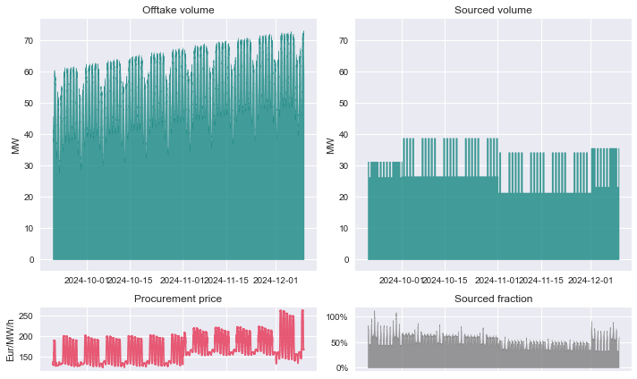
Just as when working with portfolio lines, we can get a quick overview of the portfolio state with the .plot() method…
[3]:
pfs.plot();
…and we can copy its data to the clipboard, or save it as an Excel workbook:
[4]:
pfs.to_clipboard()
pfs.to_excel("portfolio_state.xlsx")
Looking at the offtake, we can see the daily and weekly cycles, as well as a slow increase over the entire time period.
This graph is a bit too detailed for most purposes, so let’s look at the second method we know from PfLine: resampling.
Resampling
We might prefer to see hourly, daily, or monthly values instead of the quarterhourly values that are in pfs. For this, we can resample the object with the .asfreq() method. In this code example, we also use the .print() method, which adds some helpful coloring to the output:
[5]:
pfs_monthly = pfs.asfreq("MS")
pfs_monthly.print()
PfState object.
. Start: 2024-10-01 00:00:00+02:00 (incl)    . Timezone    : Europe/Berlin
. End  : 2024-12-01 00:00:00+01:00 (excl)    . Start-of-day: 00:00:00
. Freq : <MonthBegin> (2 datapoints)
                                                w           q           p             r
                                               MW         MWh     Eur/MWh           Eur
──────── offtake
           2024-10-01 00:00:00 +0200        -54.7     -40 744
           2024-11-01 00:00:00 +0100        -59.4     -42 732
─●────── pnl_cost
 │         2024-10-01 00:00:00 +0200         54.7      40 744      160.48     6 538 471
 │         2024-11-01 00:00:00 +0100         59.4      42 732      182.94     7 817 452
 ├●───── sourced
 ││        2024-10-01 00:00:00 +0200         31.2      23 221      132.58     3 078 642
 ││        2024-11-01 00:00:00 +0100         25.9      18 652      133.27     2 485 849
 │├───── quarter_products
 ││        2024-10-01 00:00:00 +0200         13.8      10 256      106.54     1 092 646
 ││        2024-11-01 00:00:00 +0100         13.7       9 897      106.78     1 056 810
 │└───── month_products
 │         2024-10-01 00:00:00 +0200         17.4      12 964      153.19     1 985 996
 │         2024-11-01 00:00:00 +0100         12.2       8 755      163.22     1 429 039
 └────── unsourced
           2024-10-01 00:00:00 +0200         23.5      17 523      197.44     3 459 829
           2024-11-01 00:00:00 +0100         33.4      24 080      221.41     5 331 603
Note how the resampled output only contains those months, that are entirely included in the original data. pfl has data in September and December, but as these are not present in their entirety, they are dropped from pfl_monthly.
On frequencies and unsourced prices
There is one other important consequence of resampling: the unsourced prices are now specific for this portfolio. We can demonstrate this by creating a second portfolio state, using the same price-forward curve (but different offtake and sourced volume):
[6]:
pfs2 = pf.PfState(offtake * 1.5, prices, sourced * 2)
At this shortest frequency, the unsourced prices are identical (namely, the price-forward curve). Let’s create a dataframe with the prices to verify this:
[7]:
pd.DataFrame(
    {"pfs": pfs.unsourcedprice.p, "pfs2": pfs2.unsourcedprice.p, "hpfc": prices.p}
)
[7]:
| pfs | pfs2 | hpfc | |
|---|---|---|---|
| 2024-09-20 00:00:00+02:00 | 139.80568207211454 | 139.80568207211454 | 139.80568207211454 |
| 2024-09-20 00:15:00+02:00 | 135.63901540544785 | 135.63901540544785 | 135.63901540544785 |
| 2024-09-20 00:30:00+02:00 | 131.47234873878116 | 131.47234873878116 | 131.47234873878116 |
| 2024-09-20 00:45:00+02:00 | 128.13901540544785 | 128.13901540544785 | 128.13901540544785 |
| 2024-09-20 01:00:00+02:00 | 124.80568207211451 | 124.80568207211451 | 124.80568207211451 |
| ... | ... | ... | ... |
| 2024-12-09 22:45:00+01:00 | 217.88078474854294 | 217.88078474854294 | 217.88078474854294 |
| 2024-12-09 23:00:00+01:00 | 221.2141180818763 | 221.2141180818763 | 221.2141180818763 |
| 2024-12-09 23:15:00+01:00 | 224.54745141520962 | 224.54745141520962 | 224.54745141520962 |
| 2024-12-09 23:30:00+01:00 | 227.88078474854294 | 227.88078474854294 | 227.88078474854294 |
| 2024-12-09 23:45:00+01:00 | 232.0474514152096 | 232.0474514152096 | 232.0474514152096 |
7780 rows × 3 columns
However, at every other frequency, they are not equal. When changing the frequency, a volume-weighted average is calculated for the unsourced prices - just like with every other price-and-volume timeseries. This makes that the unsourced prices apply only to the unsourced volume profile of that portfolio:
[8]:
pd.DataFrame(
    {
        "pfs": pfs.asfreq("MS").unsourcedprice.p,
        "pfs2": pfs2.asfreq("MS").unsourcedprice.p,
        "hpfc": prices.asfreq("MS").p,
    }
)
[8]:
| pfs | pfs2 | hpfc | |
|---|---|---|---|
| 2024-10-01 00:00:00+02:00 | 197.4437803760265 | 192.11463549822653 | 194.78888729464586 |
| 2024-11-01 00:00:00+01:00 | 221.40989836363784 | 217.79829542112196 | 220.07479863376392 |
This has important consequences.
For example, when doing a scenario analysis in which the unsourced volume is changed (e.g. “what happens if the offtake increases by 50%?”), we cannot expect the results to be correct unless we are working at the original frequency. In situations where it is clear that this error looms, a UserWarning is shown to alert the user (e.g. in the examples further below). For more information on unsourced volume, see this section in the documentation on
the PfState class.
For this reason, we commonly work with our porfolio states at the frequency of the price-forward curve. Downsampling is only done to see the aggregated values for verification or reporting.
Components
Now, let’s look at the portfolio state pfs_monthly in a bit more detail, to learn more about the PfState class.
The portfolio state is presented to us as a tree structure, with several branches. Each branch is a portfolio line. E.g, offtake and sourced are the portfolio lines we specified when creating the object. Also, the branch pnl_cost is the sum of sourced and unsourced, with sourced being the sum of quarter_products and month_products.
The unsourced volume is found by comparing the offtake to what is already sourced. This volume is valued at the market prices in the forward curve.
These portfolio lines can be obtained from the portfolio state by accessing them as attributes. E.g. .offtakevolume, .sourced, .unsourced, or .pnl_cost. The latter is the best estimate for what it will cost to procure the offtake:
[9]:
pfs_monthly.pnl_cost
[9]:
PfLine object with price and volume information.
. Start: 2024-10-01 00:00:00+02:00 (incl)    . Timezone    : Europe/Berlin
. End  : 2024-12-01 00:00:00+01:00 (excl)    . Start-of-day: 00:00:00
. Freq : <MonthBegin> (2 datapoints)
. Children: 'sourced' (price and volume), 'unsourced' (price and volume)
                                     w           q           p             r
                                    MW         MWh     Eur/MWh           Eur

2024-10-01 00:00:00 +0200         54.7      40 744      160.48     6 538 471
2024-11-01 00:00:00 +0100         59.4      42 732      182.94     7 817 452
Notice that this portfolio line has children, and as a reminder, we can “drill into” the object to get these nested portfolio line, e.g. with pfl_monthly.pnl_cost["sourced"].
There are some other components that are not explicitly shown:
We may be interested in how much of the offtake has already been sourced or unsourced. These fractions are available at the
.sourcedfractionand.unsourcedfractionproperties.You may have noticed that
unsourcedis the inverse from what traders would call the “open positions” or “portfolio positions”: if our portfolio is short, the unsourced volume is positive. For those that prefer this other perspective, it is available at.netposition.
Export
Just as with portfolio lines, we can create an excel file that contains all the information in a portfolio state with its .to_excel() method, and we can copy it to the clipboard with the .to_clipboard() method.
MtM
We can evaluate the value of our sourcing contracts against the current forward curve (“mark-to-market”) with the .mtm_of_sourced() method.
Analyses with portfolio states
We’ll now look at how we can do “what-if” analyses with portfolio state. The original portfolio state we will consider as the reference and store it in an appropriately named variable:
[10]:
ref = pfs
The monthly procurement prices of this portfolio are what interest us the most. As a reminder, we can find the procurement volumes and costs with:
[11]:
cost_ref = ref.asfreq("MS").pnl_cost
cost_ref
[11]:
PfLine object with price and volume information.
. Start: 2024-10-01 00:00:00+02:00 (incl)    . Timezone    : Europe/Berlin
. End  : 2024-12-01 00:00:00+01:00 (excl)    . Start-of-day: 00:00:00
. Freq : <MonthBegin> (2 datapoints)
. Children: 'sourced' (price and volume), 'unsourced' (price and volume)
                                     w           q           p             r
                                    MW         MWh     Eur/MWh           Eur

2024-10-01 00:00:00 +0200         54.7      40 744      160.48     6 538 471
2024-11-01 00:00:00 +0100         59.4      42 732      182.94     7 817 452
(Or we could go one step further and focus on only the prices with ref.asfreq("MS").pnl_cost.p.)
Change in offtake
Now, what would happen if the offtake were to increase by 25%? Qualitatively, this is not hard. An increase in the offtake increases the unsourced volume. And because the market prices are higher than what we pay for the sourced volume, this means that the procurement price will go up.
How much? Let’s see. First, we create a new portfolio state, from the reference, by setting the offtake to the new value. We can do this with the .set_offtake() method. After that, we can again see what the procurement volumes and costs are. (Note the UserWarning which was mentioned above.)
[12]:
higherofftake = ref.offtakevolume * 1.25
pfs_higherofftake = ref.set_offtakevolume(higherofftake)
cost_higherofftake = pfs_higherofftake.asfreq("MS").pnl_cost
cost_higherofftake
c:\users\ruud.wijtvliet\ruud\python\dev\portfolyo\portfolyo\core\pfstate\pfstate.py:199: UserWarning: This operation changes the unsourced volume. This causes inaccuracies in its price if the portfolio state has a frequency that is longer than the spot market.
  warnings.warn(
[12]:
PfLine object with price and volume information.
. Start: 2024-10-01 00:00:00+02:00 (incl)    . Timezone    : Europe/Berlin
. End  : 2024-12-01 00:00:00+01:00 (excl)    . Start-of-day: 00:00:00
. Freq : <MonthBegin> (2 datapoints)
. Children: 'sourced' (price and volume), 'unsourced' (price and volume)
                                     w           q           p             r
                                    MW         MWh     Eur/MWh           Eur

2024-10-01 00:00:00 +0200         68.4      50 930      168.64     8 588 719
2024-11-01 00:00:00 +0100         74.2      53 416      191.54    10 231 182
Comparing these two cost portfolio lines, we see that indeed the values for w and q have increased to 125% of the original values. Also, the procurement prices have increased. We can quickly calculate by how much:
[13]:
cost_higherofftake.p - cost_ref.p
[13]:
2024-10-01 00:00:00+02:00    8.160879013401626
2024-11-01 00:00:00+01:00    8.599884206454362
Freq: MS, Name: p, dtype: pint[Eur/MWh]
We could similarly create a portfolio states for situations with a market price drop of 40%. Or one which combines both effects:
[14]:
lowerprices = ref.unsourcedprice * 0.6
pfs_lowerprices = ref.set_unsourcedprice(lowerprices)
pfs_lowerprices_higherofftake = ref.set_offtakevolume(higherofftake).set_unsourcedprice(
    lowerprices
)
c:\users\ruud.wijtvliet\ruud\python\dev\portfolyo\portfolyo\core\pfstate\pfstate.py:199: UserWarning: This operation changes the unsourced volume. This causes inaccuracies in its price if the portfolio state has a frequency that is longer than the spot market.
  warnings.warn(
Hedging
Hedging can reduce the sensitivity of our portfolio to changes in the market price. Given the current market price curve, we can calculate how much we’d need to source to obtain a fully hedged portfolio:
[15]:
needed = ref.hedge_of_unsourced("val", "MS") # value hedge with month products
Let’s say we procure exactly that volume. We can add it to the sourced volume in our portfolio state:
[16]:
hedged = ref.add_sourced(pf.PfLine({"newvolume": needed}))
c:\users\ruud.wijtvliet\ruud\python\dev\portfolyo\portfolyo\core\pfstate\pfstate.py:209: UserWarning: This operation changes the unsourced volume. This causes inaccuracies in its price if the portfolio state has a frequency that is longer than the spot market.
  warnings.warn(
(We could have obtained the same result with the ref.source_unsourced() method.)
The portfolio is now hedged at the month level. We can verify this by looking at the unsourced volume. In case of a volume hedge, the unsourced volume (q and w) is 0, even if its monetary value (r) is not; in case of a value hedge, it is the reverse:
[17]:
hedged.asfreq("MS").unsourced
[17]:
PfLine object with price and volume information.
. Start: 2024-10-01 00:00:00+02:00 (incl)    . Timezone    : Europe/Berlin
. End  : 2024-12-01 00:00:00+01:00 (excl)    . Start-of-day: 00:00:00
. Freq : <MonthBegin> (2 datapoints)
                                     w           q           p             r
                                    MW         MWh     Eur/MWh           Eur

2024-10-01 00:00:00 +0200         -0.2        -173        0.00            -0
2024-11-01 00:00:00 +0100         -0.2        -134        0.00            -0
Because the market prices have not changed, the best-estimate procurement prices (at month level and longer) are also unchanged from before. (This is verified in the “before” columns of the dataframe further below.)
Market price change
A hedged profile is less impacted by market price changes. To see that this is indeed the case, let’s look at a scenario with an increase in the forward price curve by 40 Eur/MWh, for both portfolio states:
[18]:
newprices = prices + pf.Q_(40.0, "Eur/MWh")
ref_higherprices = ref.set_unsourcedprice(newprices)
hedged_higherprices = hedged.set_unsourcedprice(newprices)
The reference portfolio has gotten a lot more expensive, whereas the procurement price for the hedged portfolio has not moved significantly:
[19]:
pd.DataFrame(
    {
        ("ref", "before"): ref.pnl_cost.asfreq("MS").p,
        ("ref", "after"): ref_higherprices.pnl_cost.asfreq("MS").p,
        ("hedged", "before"): hedged.pnl_cost.asfreq("MS").p,
        ("hedged", "after"): hedged_higherprices.pnl_cost.asfreq("MS").p,
    }
).pint.dequantify()
[19]:
| ref | hedged | |||
|---|---|---|---|---|
| before | after | before | after | |
| unit | Eur/MWh | Eur/MWh | Eur/MWh | Eur/MWh |
| 2024-10-01 00:00:00+02:00 | 160.478106 | 177.681366 | 160.478106 | 160.307936 |
| 2024-11-01 00:00:00+01:00 | 182.939602 | 205.480086 | 182.939602 | 182.814260 |
For the observant reader: it may seem that the portfolio was not fully hedged after all, as a small change in the procurement price is seen. The reason is that each strategy (i.e., volume or value hedge) fully protects only against a specific price change (i.e., absolute or relative). A volume hedge does not fully hedge against an absolute price change such as the one we see here.
This tutorial is continued in part 4.