PfLine¶

The basic building block of the portfolyo package is the “portfolio line” (PfLine). Instances of this class store a timeseries containing volume information, price information, or both. This page discusses their most important properties, and how to use them.

For a tutorial, see here.

It is assumed that you are familiar with the following dimension abbrevations: w for power, q for energy, p for price, and r for revenue; see this page for more information.

Kind ¶

An important characteristic of a portfolio line is its “kind”. The property PfLine.kind has a value from the portfolyo.Kind enumeration and tells us the type of information it contains:

🟨 Kind.VOLUME: “volume-only” portfolio line.

This is a portfolio line that only contains volume information.

As an example, consider the expected/projected development of offtake volume of a customer or customer group.

The volume in each timestamp can be retrieved by the user in units of energy (e.g., MWh) or in units of power (e.g., MW).

🟩 Kind.PRICE: “price-only” portfolio line.

This is a portfolio line which only contains price information.

For example, the forward price curve for a certain market area, or the fixed offtake price that a customer is paying for a certain delivery period.
🟦 Kind.REVENUE: “revenue-only” portfolio line.

For example, the payoff of a financially-settled put option, which has a monetary value (e.g., in Eur) without an associated volume being delivered.
🟫 Kind.COMPLETE

This a portfolio line that contains volume, price and revenue information.

For example: the volume that has been sourced to hedge a certain portfolio, e.g. in monthly or quarterly blocks.

For each timestamp we have a volume (the contracted volume, both as energy and as power), a price (for which the volume was contracted) and a revenue (i.e., the multiplication of the energy and the price).

“Volume-only” and “complete” portfolio lines contain redundant information. For the volume, the power (in MW) can be calculated by dividing the energy (in MWh) by the duration of the timestamp (in h). Likewise, the price (in Eur/MWh) can be calculated by dividing the revenue (in Eur) by the energy (in MWh). See also the note in the next section.

Initialisation ¶

There are many ways to specify the timeseries from which to initialise a portfolio line; here we will discuss the most common ones. In all cases it is assumed that the data has been prepared and standardized.

In General¶

portfolyo tries to determine the dimension of information (e.g., if it is a price or a volume) using its key (if it has one) and its unit (also, if it has one) - see the section on Compatilibity of abbrevation and unit.

To initialise a volume-only / price-only / revenue-only portfolio line, we must only provide a volume / price / revenue timeseries. To initialise a complete portfolio line, we must supply at least 2 of the following timeseries: prices, volumes, revenues.

Note

Specifying volumes: it is not necessary to specify both power (w) and energy (q); for a given timestamp we can calculate one from the other. If both are specified, they should be consistent with each other.

Specifying volumes and prices: the same goes when specifying volume (either w or q), price (p) and revenue (r). Only two are needed, and if more are specified, they should be consistent.

DataFrame or dictionary of timeseries…¶

…or any other Mapping from (string) key values to pandas.Series.

The keys (or dataframe column names) must each be one of the following: w (power), q (energy), p (price), r (revenue). Depending on the keys, the .kind of the portfolio line is determined.

import portfolyo as pf
import pandas as pd
index = pd.date_range('2024', freq='YS', periods=3)
input_dict = {'w': pd.Series([200, 220, 300.0], index)}
pf.PfLine(input_dict)

PfLine object with volume information.
. Start: 2024-01-01 00:00:00 (incl)    . Timezone    : none  
. End  : 2027-01-01 00:00:00 (excl)    . Start-of-day: 00:00:00  
. Freq : <YearBegin: month=1> (3 datapoints)
                                     w           q
                                    MW         MWh

2024-01-01 00:00:00              200.0   1 756 800
2025-01-01 00:00:00              220.0   1 927 200
2026-01-01 00:00:00              300.0   2 628 000

Timeseries with unit¶

Under the condition that a valid pint unit is present, we may also provide a single timeseries (pandas.Series), or an iterable of timeseries. They are automatically converted to the default unit.

# using the imports and index from the previous example
input_series = pd.Series([10, 11.5, 10.8], index, dtype='pint[ctEur/kWh]')
pf.PfLine(input_series)

PfLine object with price information.
. Start: 2024-01-01 00:00:00 (incl)    . Timezone    : none  
. End  : 2027-01-01 00:00:00 (excl)    . Start-of-day: 00:00:00  
. Freq : <YearBegin: month=1> (3 datapoints)
                                    p
                              Eur/MWh

2024-01-01 00:00:00            100.00
2025-01-01 00:00:00            115.00
2026-01-01 00:00:00            108.00

Dictionary of portfolio lines…¶

…or any other Mapping from (string) key values to PfLine objects.

The keys are used as the children names:

pfl1 = pf.PfLine(pd.Series([0.2, 0.22, 0.3], index, dtype='pint[GW]'))
pfl2 = pf.PfLine(pd.Series([100, 150, 200.0], index, dtype='pint[MW]'))
dict_of_children = {'southeast': pfl1, 'northwest': pfl2}
pfl = pf.PfLine(dict_of_children)

PfLine object with volume information.
. Start: 2024-01-01 00:00:00 (incl)    . Timezone    : none  
. End  : 2027-01-01 00:00:00 (excl)    . Start-of-day: 00:00:00  
. Freq : <YearBegin: month=1> (3 datapoints)
. Children: 'southeast' (volume), 'northwest' (volume)
                                     w           q
                                    MW         MWh

2024-01-01 00:00:00              300.0   2 635 200
2025-01-01 00:00:00              370.0   3 241 200
2026-01-01 00:00:00              500.0   4 380 000

Note that the aggregate values are shown.

Nesting is not limited to one level, and, instead of having each value be a PfLine objects, it is actually sufficient that each value can be used to initialise a PfLine object.

Flat or Nested ¶

As seen in the final initialisation example, we can create nested portfolio lines, where a portfolio line contains one or more named children (which are also portfolio lines). This in contrast to the ‘flat’ portfolio lines we created in the first initialisation example.

Note

When checking the types, you will see that these are actually different classes - in the examples above FlatVolumePfLine, FlatPricePfLine, and NestedVolumePfLine. All are descendents of the PfLine base class. When initialising a PfLine, the correct type will be returned based on the input data.

For nested portfolio lines, we are always looking at and working with the the top level, i.e., the sum/aggregate - unless explicitly requested otherwise by the user.

An example of where a nested portfolio line makes sense, is to combine procurement on the forward market and spot trade into a single “sourced” portfolio line. We can then easily work with the aggregate values, but the values of the individual markets are also still available.

It is important to note that both types of portfolio line contain the exact same methods and properties that are described in the rest of this document. Nested portfolio lines do have a few additional methods which are described now.

Working with children¶

The following common operations on nested portfolio lines are implemented:

We can access a particular child by using its name as an index, e.g. pfl['southeast']. If it does not collide with any of the attribute names, we can also access it by attribute, e.g. pfl.southeast.
We can iterate over all children with for name in pfl or for (name, child) in pfl.items().
We can add a new child to a portfolio with pfl_new = pfl.set_child('southwest', ...). this returns a reference to the new object; the original object is unchanged. (It is immutable by design.)
Likewise, we can remove a child from the portfolio with pfl_new = pfl.drop_child('southeast'). At least one child should remain.
If we are no longer interested in the particulars of each child, we can keep only the top-level information with the .flatten() method, which returns a flattened copy of the object.

Note that a portfolio line may quietly be flattened whenever an operation is done that is ambiguous or undefined for a portfolio line with children. See the section on arithmatic below.

Accessing data ¶

In order to get our data out of a portfolio line, the following options are available.

Timeseries¶

The properties PfLine.w, .q, .p and .r always return the information as a pandas.Series. These have a pint unit, which can be stripped using .pint.m (or .pint.magnitude).

import portfolyo as pf, pandas as pd
index = pd.date_range('2024', freq='YS', periods=3)
input_df = pd.DataFrame({'w':[200, 220, 300], 'p': [100, 150, 200]}, index)
pfl = pf.PfLine(input_df)

pfl.r

2024-01-01    175680000.0
2025-01-01    289080000.0
2026-01-01    525600000.0
Freq: YS-JAN, Name: r, dtype: pint[Eur]

DataFrame¶

If we want to extract more than one timeseries, we can use the .df attribute, which contains all relevant (top-level) timeseries.

# continuation of previous code example
pfl.df

                w          q      p            r
2024-01-01  200.0  1756800.0  100.0  175680000.0
2025-01-01  220.0  1927200.0  150.0  289080000.0
2026-01-01  300.0  2628000.0  200.0  525600000.0

We can also use the .dataframe() method, which has a few options to control the exact format and contents of the dataframe.

Index¶

The PfLine.index property returns the pandas.DatetimeIndex that applies to the data. This includes the frequency that tells us how long the time periods are that start at each of the timestamps in the index.

# continuation of previous code example
pfl.index

DatetimeIndex(['2024-01-01', '2025-01-01', '2026-01-01'], dtype='datetime64[ns]', freq='YS-JAN')

For convenience, portfolyo adds a .duration and a right property to the pandas.DatetimeIndex class, which do as we would predict:

# continuation of previous code example
pfl.index.duration, pfl.index.right

2024-01-01    8784.0
2025-01-01    8760.0
2026-01-01    8760.0
Freq: YS-JAN, Name: duration, dtype: pint[h] 
 DatetimeIndex(['2025-01-01', '2026-01-01', '2027-01-01'], dtype='datetime64[ns]', name='right', freq='YS-JAN')

Index slice¶

From pandas we know the .loc[] property which allows us to select a slice of the objects. This is implemented also for portfolio lines. Currently, it supports enering a slice of timestamps. It is a wrapper around the pandas.DataFrame.loc[] property, and therefore follows the same convention, with the end point being included in the result.

Another slicing method is implemented with the .slice[] property. The improvement to .loc[] is, that .slice[] uses the more common convention of excluding the end point. This has several advantages, which stem from the fact that, unlike when using .loc, using left = pfl.slice[:a] and right = pfl.slice[a:] returns portfolio lines that are complements - every timestamp in the original portfolio line is found in either the left or the right slice. This is useful when e.g. concatenating portfolio lines (see below.)

# continuation of previous code example
pfl.slice['2024':'2026']  # excludes 2026; 2026 interpreted as timestamp 2026-01-01 00:00:00

PfLine object with complete information.
. Start: 2024-01-01 00:00:00 (incl)    . Timezone    : none  
. End  : 2026-01-01 00:00:00 (excl)    . Start-of-day: 00:00:00  
. Freq : <YearBegin: month=1> (2 datapoints)
                                     w           q           p             r
                                    MW         MWh     Eur/MWh           Eur

2024-01-01 00:00:00              200.0   1 756 800      100.00   175 680 000
2025-01-01 00:00:00              220.0   1 927 200      150.00   289 080 000

Reindexing¶

A portfolio line can be reindexed with .index(), using another index, e.g. of another portfolio line. This returns a new portfolio line, with the specified index. Any timestamps that were not present in the original object are filled with “zero” (as applicable).

# continuation of previous code example
index2 = pd.date_range('2025', freq='YS', periods=3)
pfl.reindex(index2)  # 2024 is dropped; 2025 and 2026 are kept; 2027 is new (0)

PfLine object with complete information.
. Start: 2025-01-01 00:00:00 (incl)    . Timezone    : none  
. End  : 2028-01-01 00:00:00 (excl)    . Start-of-day: 00:00:00  
. Freq : <YearBegin: month=1> (3 datapoints)
                                     w           q           p             r
                                    MW         MWh     Eur/MWh           Eur

2025-01-01 00:00:00              220.0   1 927 200      150.00   289 080 000
2026-01-01 00:00:00              300.0   2 628 000      200.00   525 600 000
2027-01-01 00:00:00                0.0           0                         0

Concatenation¶

Portfolio lines can be concatenated with the portfolio.concat() function. This only works if the input portfolio lines have contain compatible information (the same frequency, timezone, start-of-day, kind, etc) and, crucially, their indices are gapless and without overlap. To remove any overlap, use the .slice[] property.

# continuation of previous code example
index2 = pd.date_range('2025', freq='YS', periods=3)  # 2 years' overlap with pfl
pfl2 = pf.PfLine(pd.DataFrame({'w':[22, 30, 40], 'p': [15, 20, 21]}, index))
# first two datapoints (until/excl 2026) from pfl, last two datapoints (from/incl 2026) from pfl2
pf.concat([pfl.slice[:'2026'], pfl2.slice['2026':]])

PfLine object with complete information.
. Start: 2024-01-01 00:00:00 (incl)    . Timezone    : none  
. End  : 2027-01-01 00:00:00 (excl)    . Start-of-day: 00:00:00  
. Freq : <YearBegin: month=1> (3 datapoints)
                                     w           q           p             r
                                    MW         MWh     Eur/MWh           Eur

2024-01-01 00:00:00              200.0   1 756 800      100.00   175 680 000
2025-01-01 00:00:00              220.0   1 927 200      150.00   289 080 000
2026-01-01 00:00:00               40.0     350 400       21.00     7 358 400

Volume-only, price-only or revenue-only¶

With the .volume, .price and .revenue properties, we are able to extract the specified data from a complete portfolio line. For nested portfolios lines, the returned PfLine may still be flat; this is the case if keeping the children would lead to incorrect values. (E.g., getting the price part of a nested complete portfolio line: the aggregate price is the average of the children’s prices, weighted with their volumes. The individual prices cannot simply be added up.)

Further below, in the section on arithmatic, we see the reverse operation: combining two portfolio lines into a complete one.

Plotting / Excel / Clipboard ¶

There are several ways to get data into other formats.

Plotting¶

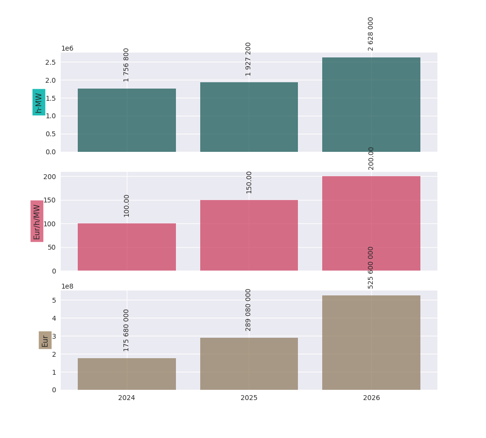
The data can be shown graphically with the .plot() method:

# continuation of previous code example
pfl.plot()

Excel and clipboard¶

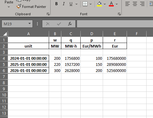
Often, further data analyses are done in Excel. If you have a Workbook open, the easiest way is to copy the portfolio line data to the clipboard with the .to_clipboard() method. From there, it can be pasted onto a worksheet.

Alternatively, the data can be saved as an Excel workbook with the .to_excel() method.

# continuation of previous code example
pfl.to_clipboard()
pfl.to_excel("sourced_volume.xlsx")

Resampling ¶

Using the .asfreq() method, we can quickly and correctly downsample our data, e.g. to monthly or yearly values. For price-and-volume portfolio lines, the prices are weighted with the energy as one would expect:

# continuation of previous code example
pfl.asfreq('QS')

PfLine object with complete information.
. Start: 2024-01-01 00:00:00 (incl)    . Timezone    : none  
. End  : 2027-01-01 00:00:00 (excl)    . Start-of-day: 00:00:00  
. Freq : <QuarterBegin: startingMonth=1> (12 datapoints)
                                     w           q           p             r
                                    MW         MWh     Eur/MWh           Eur

2024-01-01 00:00:00              200.0     436 800      100.00    43 680 000
2024-04-01 00:00:00              200.0     436 800      100.00    43 680 000
2024-07-01 00:00:00              200.0     441 600      100.00    44 160 000
2024-10-01 00:00:00              200.0     441 600      100.00    44 160 000
2025-01-01 00:00:00              220.0     475 200      150.00    71 280 000
2025-04-01 00:00:00              220.0     480 480      150.00    72 072 000
2025-07-01 00:00:00              220.0     485 760      150.00    72 864 000
2025-10-01 00:00:00              220.0     485 760      150.00    72 864 000
2026-01-01 00:00:00              300.0     648 000      200.00   129 600 000
2026-04-01 00:00:00              300.0     655 200      200.00   131 040 000
2026-07-01 00:00:00              300.0     662 400      200.00   132 480 000
2026-10-01 00:00:00              300.0     662 400      200.00   132 480 000

For more information about resampling in general, see this page.

Arithmatic ¶

There are many ways to change and interact with PfLine instances. An intuitive way is through arithmatic, described below. The operations are grouped by the operator, and colors are used to more easily indicate the type of the output value.

General remarks:

The operands are defined liberally. E.g. “price” means any object that can be interpreted as a price: a single pint.Quantity with a valid price unit; a pandas.Series with a pint unit of price, a dictionary with a single key "p", a pandas.Dataframe with a single column "p", or a price-only portfolio line; see Interoperability.

The following code example shows a few equivalent operations.

import portfolyo as pf, pandas as pd
index = pd.date_range('2024', freq='YS', periods=3)
pfl = pf.PfLine(pd.Series([2, 2.2, 3], index, dtype='pint[MW]'))
pfl_1 = pfl + {'q': 50.0}  # standard unit (here: MWh) is assumed
pfl_2 = pfl + pf.Q_(50000.0, 'kWh')
pfl_3 = pfl + {'q': pd.Series([50, 50, 50.0], index)}
pfl_4 = pfl + pf.PfLine({'q': pd.Series([50, 50, 50.0], index)})
pfl_1 == pfl_2 == pfl_3 == pfl_4

True

If two portfolio lines span distinct periods, only their overlap is kept. If instead we want to keep all timestamps, e.g., when adding a portfolio line which spans a quarter to one that spans a year (with the same frequency, e.g. hourly), first use the .reindex() method on the former with the index of the latter. The values outside the specified quarter are filled with “zero” values as is applicable to the kind of portfolio line under consideration.
A single value is understood to apply uniformly to each timestamp in the index of the portfolio line.
When doing arithmatic with a flat portfolio line, the result is again a flat portfolio line.
When doing arithmatic with a nested portfolio line, the children are also present in the result.
Arithmatic does silent flattening if necessary. E.g., if an operation is only possible if one or both of the operands is flat, this will be done automatically. (A nested portfolio line can also be flattened manually with the .flatten() method.)
However, an Exception is raised in case of ambiguity concerning the unit. E.g., when adding a float value to a PRICE portfolio line. Solution: explicitly convert into a pint.Quantity using pf.Q_().
The usual relationship between addition and multiplication holds. E.g., for a given portfolio line pfl, the following two calculations have the same return value: pfl + pfl and 2 * pfl.

Addition and subtraction¶

Addition and subtraction are only possible between operands of the same kind. E.g., to a price-only portfolio line, a price can be added, but not e.g. a volume.
Even if the both operands have the same kind, they must both be nested or both be flat. E.g., a flat price can be added to a flat price-only portfolio line, but not to a nested price-only portfolio line. Two nested price-only portfolio lines can be added.

	Kind of portfolio line (pfl.Kind)
	🟨 `VOLUME`	🟩 `PRICE`	🟦 `REVENUE`	🟫 `COMPLETE`
`pfl` ± volume	🟨 e	❌	❌	❌
`pfl` ± price	❌	🟩 e	❌	❌
`pfl` ± revenue	❌	❌	🟦 e	❌
`pfl` ± complete	❌	❌	❌	🟫 e

Notes:

e: “Equal”: both operands must be flat or both must be nested.

Here are several examples.

Adding a volume to a volume-only portfolio line:

import portfolyo as pf, pandas as pd
index = pd.date_range('2024', freq='YS', periods=3)
vol = pf.PfLine(pd.Series([4, 4.6, 3], index, dtype='pint[MW]'))
vol + pf.Q_(10.0, 'GWh')

PfLine object with volume information.
. Start: 2024-01-01 00:00:00 (incl)    . Timezone    : none  
. End  : 2027-01-01 00:00:00 (excl)    . Start-of-day: 00:00:00  
. Freq : <YearBegin: month=1> (3 datapoints)
                                     w           q
                                    MW         MWh

2024-01-01 00:00:00                5.1      45 136
2025-01-01 00:00:00                5.7      50 296
2026-01-01 00:00:00                4.1      36 280

When adding (or subtracting) two nested portfolio lines, the children are merged:

# continuation of previous code example
vol_2 = pf.PfLine({
    'A': pd.Series([4, 4.6, 3], index, dtype='pint[MW]'),
    'B': pd.Series([1, -1.8, 1.9], index, dtype='pint[MW]')
})
vol_3 = pf.PfLine({
    'B': pd.Series([0.5, 0.2, 1.9], index, dtype='pint[MW]'),
    'C': pd.Series([2, 2.2, 3.8], index, dtype='pint[MW]')
})
diff = vol_2 - vol_3

print([name for name in diff])
diff['B']

['C', 'B', 'A']

PfLine object with volume information.
. Start: 2024-01-01 00:00:00 (incl)    . Timezone    : none  
. End  : 2027-01-01 00:00:00 (excl)    . Start-of-day: 00:00:00  
. Freq : <YearBegin: month=1> (3 datapoints)
                                     w           q
                                    MW         MWh

2024-01-01 00:00:00                0.5       4 392
2025-01-01 00:00:00               -2.0     -17 520
2026-01-01 00:00:00                0.0           0

A flat and a nested portfolio line cannot be added…

…and if we try, the nested one is flattened (and the result is also a flat portfolio line):

# continuation of previous code example
vol + vol_2

If we want, we can keep the children. In that case, we must give the flat one a name as well (and the result is a nested portfolio line):

# continuation of previous code example
vol_2 + {'D': vol}

PfLine object with volume information.
. Start: 2024-01-01 00:00:00 (incl)    . Timezone    : none  
. End  : 2027-01-01 00:00:00 (excl)    . Start-of-day: 00:00:00  
. Freq : <YearBegin: month=1> (3 datapoints)
. Children: 'A' (volume), 'D' (volume), 'B' (volume)
                                     w           q
                                    MW         MWh

2024-01-01 00:00:00                9.0      79 056
2025-01-01 00:00:00                7.4      64 824
2026-01-01 00:00:00                7.9      69 204

Scaling¶

We can scale a portfolio line by multiplication with / division by a dimensionless (e.g. float) value.

This applied to flat and nested portfolio line, regardless of the kind.
The result is a portfolio line of the same kind.
If the portfolio line is nested, the scaling applies to all children.
For complete portfolio lines, the volume and revenue are scaled, while the price remains unchanged.

Negation is implemented as multiplication with -1.

	Kind of portfolio line (pfl.Kind)
	🟨 `VOLUME`	🟩 `PRICE`	🟦 `REVENUE`	🟫 `COMPLETE`
`-pfl` (negation)	🟨	🟩	🟦	🟫
`pfl * dimensionless`	🟨	🟩	🟦	🟫
`pfl / dimensionless`	🟨	🟩	🟦	🟫

For example:

import portfolyo as pf, pandas as pd
index = pd.date_range('2024', freq='MS', periods=3)
vol = pf.PfLine(pd.Series([100, 250, 100], index, dtype='pint[MW]'))
vol * 2  # multiplication with factor results in scaled portfolio line

PfLine object with volume information.
. Start: 2024-01-01 00:00:00 (incl)    . Timezone    : none  
. End  : 2024-04-01 00:00:00 (excl)    . Start-of-day: 00:00:00  
. Freq : <MonthBegin> (3 datapoints)
                                     w           q
                                    MW         MWh

2024-01-01 00:00:00              200.0     148 800
2024-02-01 00:00:00              500.0     348 000
2024-03-01 00:00:00              200.0     148 800

Calculating ratio¶

We can calculate the ratio of two portfolyo lines by dividing them.

The portfolio lines must both be flat, and of the same kind.
The result is a dimensionless pandas.Series.
None of the operands may be nested. First .flatten() if necessary.
None of the operands may be a complete portfolio line. First select the .volume, .price or .revenue if necessary.

	Kind of portfolio line (pfl.Kind)
	🟨 `VOLUME`	🟩 `PRICE`	🟦 `REVENUE`	🟫 `COMPLETE`
`pfl / volume`	⬛️ 2f	❌	(❌)	❌
`pfl / price`	❌	⬛️ 2f	(❌)	❌
`pfl / revenue`	❌	❌	⬛️ 2f	❌

Notes:

2f: Both operands must be flat.
(❌): This operation is allowed but does not result in a ratio. It is described in the section changekind below.

For example:

# continuation of previous code example
vol / pf.Q_(200.0, 'MW')  # division by volume results in dimensionless series

2024-01-01     0.5
2024-02-01    1.25
2024-03-01     0.5
Freq: MS, Name: fraction, dtype: pint[]

Changing kind¶

We can turn one kind of portfolio line into another kind, by multiplying with or division by the correct (third) kind.

Concrete, because price * volume = revenue, we have these possibilities:
- Multiplying a volume portfolio line with a price portfolio line results in a revenue portfolio line.
- Dividing a revenue portfolio line by a price portfolio line results in a volume portfolio line.
- Dividing a revenue portfolio line by a volume portfolio line results in a price portfolio line.
At most one of the operands may be nested. First .flatten() if necessary.
If one of the operands is nested, the value of the flat operand is combined with each child of the nested one.
None of the operands may be a complete portfolio line. First select the .volume, .price or .revenue if necessary.
To combine two portfolio lines into a complete portfolio line, see the section Union into complete portfolio line, below.

	Kind of portfolio line (pfl.Kind)
	🟨 `VOLUME`	🟩 `PRICE`	🟦 `REVENUE`	🟫 `COMPLETE`
`pfl * volume`	❌	🟦 ≥1f	❌	❌
`pfl * price`	🟦 ≥1f	❌	❌	❌
`pfl / volume`	(❌)	❌	🟩 ≥1f	❌
`pfl / price`	❌	(❌)	🟨 ≥1f	❌

Notes:

≥1f: At least one of the operands must be flat.
(❌): This operation is allowed but results in a ratio. It is described in the section Calculating ratio above.

Here is an examples:

# continuation of previous code example
vol * pf.Q_(100.0, 'Eur/MWh')  # multiplication with price results in revenue

PfLine object with revenue information.
. Start: 2024-01-01 00:00:00 (incl)    . Timezone    : none  
. End  : 2024-04-01 00:00:00 (excl)    . Start-of-day: 00:00:00  
. Freq : <MonthBegin> (3 datapoints)
                                      r
                                    Eur

2024-01-01 00:00:00           7 440 000
2024-02-01 00:00:00          17 400 000
2024-03-01 00:00:00           7 440 000

Union into complete portfolio line¶

We can combine portfolio lines of distinct kind into a complete portfolio line. We use the union operator | for this.

None of the operands may be a complete portfolio line. First select the .volume, .price or .revenue if necessary.
Both operands must be flat. If necessary, first .flatten() a nested portfolio line.

	Kind of portfolio line (pfl.Kind)
	🟨 `VOLUME`	🟩 `PRICE`	🟦 `REVENUE`	🟫 `COMPLETE`
`pfl \| volume`	❌	🟫 2f⠀	🟫 2f⠀	❌
`pfl \| price`	🟫 2f⠀	❌	🟫 2f⠀	❌
`pfl \| revenue`	🟫 2f⠀	🟫 2f⠀	❌	❌

2f: Both operands must be flat.

Example with flat portfolio lines:

# continuation of previous code example
vol | pf.Q_(100.0, 'Eur/MWh')  # union with price results in complete portfolio line

PfLine object with complete information.
. Start: 2024-01-01 00:00:00 (incl)    . Timezone    : none  
. End  : 2024-04-01 00:00:00 (excl)    . Start-of-day: 00:00:00  
. Freq : <MonthBegin> (3 datapoints)
                                     w           q           p             r
                                    MW         MWh     Eur/MWh           Eur

2024-01-01 00:00:00              100.0      74 400      100.00     7 440 000
2024-02-01 00:00:00              250.0     174 000      100.00    17 400 000
2024-03-01 00:00:00              100.0      74 400      100.00     7 440 000

Set timeseries ¶

Sometimes we may want to replace one part of a PfLine, while keeping the others the same. For this, first select the part we want to keep, and then use the union operator to combine it with the wanted quantity. E.g.: pfl.volume | pf.Q_(100, 'Eur/MWh')

Hedging ¶

In general, hedging is the act of reducing the exposure to certain risks. In power and gas portfolios, it is common for customers to pay a fixed, pre-agreed price for the volume they consume. By sourcing volume on the market as soon as a customer is acquired, the open positions can be kept small, effectively hedging the portfolio’s profit against market price changes.

A perfect hedge would be to buy the exact offtake volume of a portfolio in every delivery period at the shortest time-scale, e.g., days for gas and (quarter) hours for power. This is usually not possible, and hedging is done with standard products instead. Depending on the time until delivery, these may be month, quarter, or year bands; in power these exists for base, peak, and offpeak.

Using the .hedge_with() method, the volume timeseries in a portfolio line is compared with a price timeseries, and the corresponding portfolio line in standard products is returned. Parameters specify the forward price curve, the length of the products (e.g. months), the hedge method (volume hedge or value hedge), and whether to use a base band or split in peak and offpeak values.

import portfolyo as pf, pandas as pd
index = pd.date_range('2024-04-01', '2024-06-01', freq='h', inclusive='left')
offtake = pf.PfLine(pf.dev.w_offtake(index))  # mock offtake volumes
prices = pf.PfLine(pf.dev.p_marketprices(index)) # mock market prices
# Create hedge
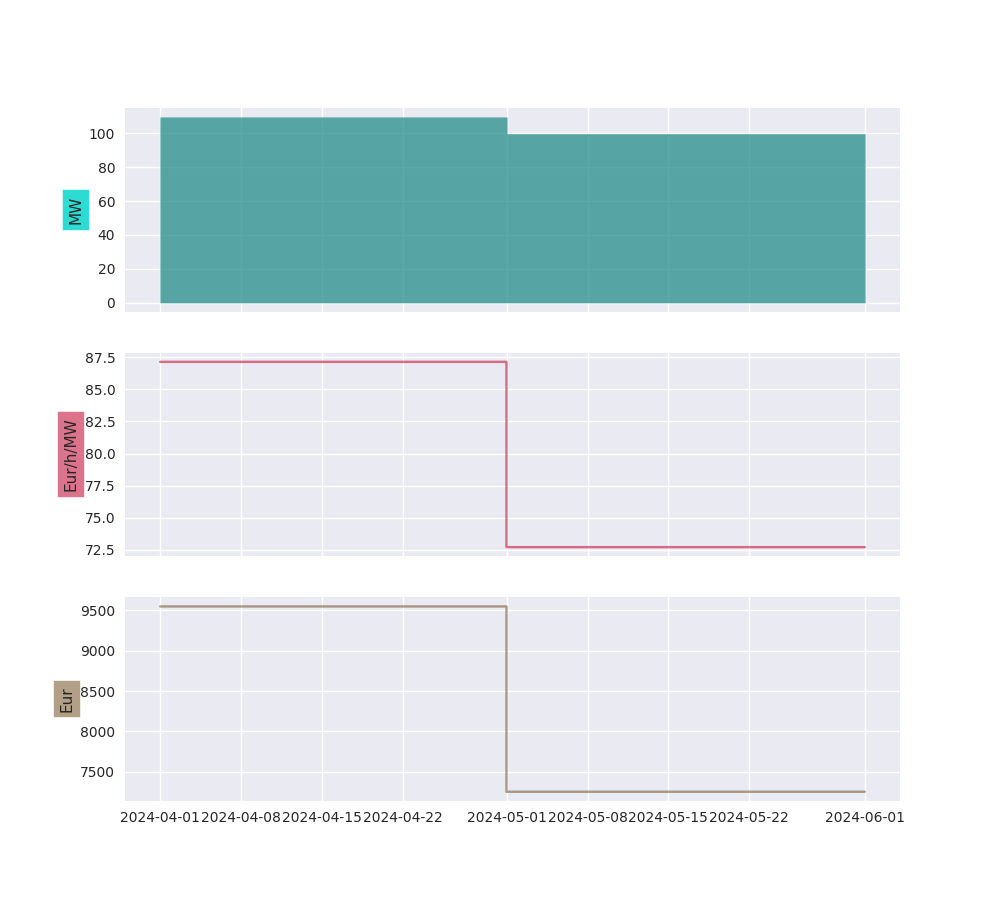
hedge = offtake.hedge_with(prices, 'vol')
# Compare the two:
(offtake | prices).plot()
hedge.plot()

Peak and offpeak ¶

For markets that have a concept of “peak” and “offpeak” periods, the .po() method splits the values in peak and offpeak. We need to specifiy a PeakFunction to determine which periods are peak - we can create one with portfolyo.create_peakfn(), or we use the one for the German power market which is provided under portfolyo.germanpower_peakfn. We can again specify if we want monthly, quarterly, or yearly values.

# continuation of previous code example
offtake.po(pf.germanpower_peakfn)

                    duration                   q                   w
2024-04-01 peak        264.0  33317.679366836615  126.20333093498718
           offpeak     456.0   45597.88306463254   99.99535759787837
2024-05-01 peak        276.0  31969.613247278034   115.8319320553552
           offpeak     468.0   42306.28521664748   90.39804533471683

NB: be cautious in using the output of this method. The values in the “sub-dataframes” do not apply to the entire time period, so the usual relations (e.g. energy = power * duration) do not hold if the duration of the entire time period is used. For convenience, the relevant duration (of only the peak or only the offpeak hours) is included in the dataframe.

API ¶

class portfolyo.PfLine(data=None, *args, **kwargs)¶

Class to hold a related energy timeseries. This can be volume data (with q [MWh] and w [MW]), price data (with p [Eur/MWh]), revenue data (with r [Eur]), or a combination of all.

abstract asfreq(freq: str = 'MS') → NDFrameLike¶

Resample the instance to a new frequency.

Parameters:: freq (str, optional) – The frequency at which to resample. ‘YS’ for year, ‘QS’ for quarter, ‘MS’ (default) for month, ‘D for day’, ‘h’ for hour, ‘15min’ for quarterhour.
Returns:: Resampled at wanted frequency.
Return type:: Instance

abstract dataframe(cols: Iterable[str] | None = None, has_units: bool = True, *args, **kwargs) → DataFrame¶

DataFrame for portfolio line in default units.

Parameters:

cols (str, optional (default: all that are available)) – The columns (w, q, p, r) to include in the dataframe. Columns that are not available are silently excluded.
has_units (bool, optional (default: True)) –
- If True, return dataframe with pint units. (The unit can be extracted
  as a column level with .pint.dequantify()).
- If False, return dataframe with float values.

Return type:

pd.DataFrame

property end: Timestamp¶: End (excl) of the portfolio line.

abstract flatten() → PfLine¶: Return flattened instance, i.e., without children.

abstract hedge_with(p: PricePfLine, how: str = 'val', peak_fn: Callable[[DatetimeIndex], Series] | None = None, freq: str = 'MS') → PfLine¶

Hedge the volume in the portfolio line with a price curve.

Parameters:

p (PricePfLine) – Portfolio line with prices to be used in the hedge.
how (str, optional (Default: 'val')) – Hedge-constraint. ‘vol’ for volumetric hedge, ‘val’ for value hedge.
peak_fn (PeakFunction, optional (default: None)) – To hedge with peak and offpeak products: function that returns boolean Series indicating if timestamps in index lie in peak period. If None, hedge with base products.
freq ({'D' (days), 'MS' (months, default), 'QS' (quarters), 'YS' (years)}) – Frequency of hedging products. E.g. ‘QS’ to hedge with quarter products.