Tutorial part 1
In this first part, we’ll look at the PfLine class.
Imports and example data
We start by importing the package. In this tutorial we will always be using the pf alias. We also import pandas with its common alias pd.
[1]:
import portfolyo as pf
import pandas as pd
For real-life applications, our input data will likely be a pandas.Series or pandas.DataFrame, read from an Excel workbook, database, or other data service. Before this data can be used, it must often be “standardized” so that it has a certain format. That is not part of this tutorial; see this section for more information on standardizing input data.
In order to get some data “to play with”, portfolyo has a few mock functions which we will use in this tutorial. Let’s get some example data for 2024 in daily resolution, as a pandas.Series:
[2]:
index = pd.date_range("2024", freq="D", periods=366)
ts_offtake = -1 * pf.dev.w_offtake(index)
ts_offtake
[2]:
2024-01-01    -109.48562536181115
2024-01-02     -117.4094985644938
2024-01-03    -119.41091107114026
2024-01-04    -116.78013138698311
2024-01-05    -119.51185255554175
                     ...
2024-12-27    -117.70326661059724
2024-12-28    -111.33880609787134
2024-12-29     -98.00848038750523
2024-12-30    -111.01554999345562
2024-12-31    -119.57010826865002
Freq: D, Name: w, Length: 366, dtype: pint[MW]
The “w” in w_offtake indicates that the timeseries has power values, which we can also see by the dtype == "pint[MW]". See this section on dimensions and units for more information.
(If our data source provides timeseries of floats, i.e., without a unit, we can explicitly set the unit with .astype("pint[MW]").)
Sign conventions are a touchy subject for portfolio managers; in this case, the function returns positive values, and we flip the sign to indicate that this volume leaves the portfolio.
My first portfolio line
One of the main classes defined by portfolyo is the PfLine (portfolio line).
Initialisation
We can initialise one with the offtake timeseries by passing it as a dictionary value. The corresponding key "w" indicates that we are dealing with power values:
[3]:
offtake = pf.PfLine({"w": ts_offtake})
offtake
[3]:
PfLine object with volume information.
. Start: 2024-01-01 00:00:00 (incl)    . Timezone    : none
. End  : 2025-01-01 00:00:00 (excl)    . Start-of-day: 00:00:00
. Freq : <Day> (366 datapoints)
                                     w           q
                                    MW         MWh

2024-01-01 00:00:00             -109.5      -2 628
2024-01-02 00:00:00             -117.4      -2 818
2024-01-03 00:00:00             -119.4      -2 866
2024-01-04 00:00:00             -116.8      -2 803
2024-01-05 00:00:00             -119.5      -2 868
2024-01-06 00:00:00             -110.8      -2 659
2024-01-07 00:00:00             -100.9      -2 422
2024-01-08 00:00:00             -113.4      -2 721
2024-01-09 00:00:00             -117.5      -2 821
2024-01-10 00:00:00             -119.1      -2 858
..                                  ..          ..
2024-12-23 00:00:00             -109.5      -2 628
2024-12-24 00:00:00             -117.4      -2 817
2024-12-25 00:00:00             -115.7      -2 777
2024-12-26 00:00:00             -116.8      -2 803
2024-12-27 00:00:00             -117.7      -2 825
2024-12-28 00:00:00             -111.3      -2 672
2024-12-29 00:00:00              -98.0      -2 352
2024-12-30 00:00:00             -111.0      -2 664
2024-12-31 00:00:00             -119.6      -2 870
There are 3 kinds of portfolio line. The one above is a volume-only portfolyo line, and this volume is shown both as power w in [MW] and as energy q in [MWh].
We can create a similar portfolio line containing price-only data:
[4]:
ts_prices = pf.dev.p_marketprices(index)
prices = pf.PfLine({"p": ts_prices})
The third kind is a price-and-volume portfolio line. We can create this, either directly (e.g. by initialising a PfLine with a dictiory having both an 'q' and 'r' key), or through arithmatic (see below).
Let’s have a look at some of the features of the PfLine class.
Plotting
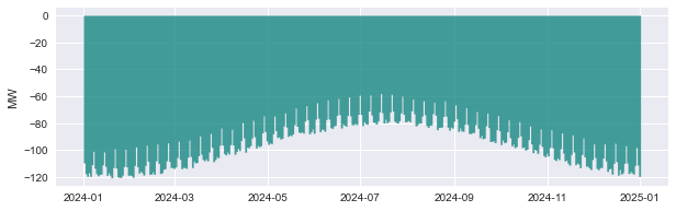
A good first look at the data is graphically. For this we can use the .plot() method:
[5]:
offtake.plot();
Resampling
Often we will want to aggregate the data to another frequency. For this we can use the .asfreq() method, e.g., to get quarterly values:
[6]:
prices.asfreq("QS")
[6]:
PfLine object with price information.
. Start: 2024-01-01 00:00:00 (incl)    . Timezone    : none
. End  : 2025-01-01 00:00:00 (excl)    . Start-of-day: 00:00:00
. Freq : <QuarterBegin: startingMonth=1> (4 datapoints)
                                    p
                              Eur/MWh

2024-01-01 00:00:00            120.90
2024-04-01 00:00:00             82.44
2024-07-01 00:00:00             78.99
2024-10-01 00:00:00            117.56
(portfolyo ensures that the values are aggregated correctly. In this case, the price (p) values are weighted-averaged (weighted with the duration of each datapoint - in this case a uniform 24h). See Resampling for more information.)
The argument "QS" specifies that we want quarterly values starting from January (same as "QS-JAN"). The allowed values, in increasing duration, are following: "15min" (=quarterhourly), "h" (=hourly), "D" (=daily), "MS" (=monthly), "QS" (=quarterly, or "QS-FEB", "QS-MAR", etc.), or "YS" (=yearly, or "YS-FEB", "YS-MAR", etc.).
Extracting data
If we want to extract the data in a portfolio line, we have several options.
Firstly, we can obtain well-known pandas.Series, with the properties .w, .q, .p, .r. For the offtake portfolio line, only .w and .q return non-NaN-values; for the price portfolio line, it is only .p:
[8]:
prices.p
[8]:
2024-01-01    134.47496375578058
2024-01-02    133.29093392195819
2024-01-03    129.28921635861454
2024-01-04    125.48318601110948
2024-01-05     124.7388613599846
                     ...
2024-12-27    123.37095664514214
2024-12-28    126.24882933415036
2024-12-29    130.58180253056403
2024-12-30    133.10705904093814
2024-12-31    131.92302920711575
Freq: D, Name: p, Length: 366, dtype: pint[Eur/MW/h]
As can be seen from the data type, this series includes the unit (using the pint package), but this can be easily stripped with .pint.m, returning a plain timeseries of floats.
We can also obtain a pandas.DataFrame with the .df() method. Here too the unit is included. In this case, it can be stripped (and inserted as a column level) with .pint.dequantify(), as demonstrated here:
[9]:
offtake.df().pint.dequantify()
[9]:
| w | q | |
|---|---|---|
| unit | MW | MW·h |
| 2024-01-01 | -109.485625 | -2627.655009 |
| 2024-01-02 | -117.409499 | -2817.827966 |
| 2024-01-03 | -119.410911 | -2865.861866 |
| 2024-01-04 | -116.780131 | -2802.723153 |
| 2024-01-05 | -119.511853 | -2868.284461 |
| ... | ... | ... |
| 2024-12-27 | -117.703267 | -2824.878399 |
| 2024-12-28 | -111.338806 | -2672.131346 |
| 2024-12-29 | -98.008480 | -2352.203529 |
| 2024-12-30 | -111.015550 | -2664.373200 |
| 2024-12-31 | -119.570108 | -2869.682598 |
366 rows × 2 columns
Finally, we can export the data to an Excel workbook with the .to_excel() method, or copy it to the clipboard (to be pasted into e.g. Excel) with the .to_clipboard() method:
[10]:
offtake.to_clipboard()
Arithmatic with portfolio lines
We can do arithmatic with portfolio line. For details on what is possible and which are the return values, see the table here.
A useful function is pf.Q_(), which returns a single pint.Quantity and understands various units:
[11]:
pf.Q_(200.0, "MW") == pf.Q_(0.2, "GW") == pf.Q_(12.0, "GJ/min")
[11]:
True
Adding / Subtracting fixed value
We can increase the offtake by a uniform 200 MW like so: (- due to the offtake being negative.)
[12]:
offtake - pf.Q_(0.2, "GW")
[12]:
PfLine object with volume information.
. Start: 2024-01-01 00:00:00 (incl)    . Timezone    : none
. End  : 2025-01-01 00:00:00 (excl)    . Start-of-day: 00:00:00
. Freq : <Day> (366 datapoints)
                                     w           q
                                    MW         MWh

2024-01-01 00:00:00             -309.5      -7 428
2024-01-02 00:00:00             -317.4      -7 618
2024-01-03 00:00:00             -319.4      -7 666
2024-01-04 00:00:00             -316.8      -7 603
2024-01-05 00:00:00             -319.5      -7 668
2024-01-06 00:00:00             -310.8      -7 459
2024-01-07 00:00:00             -300.9      -7 222
2024-01-08 00:00:00             -313.4      -7 521
2024-01-09 00:00:00             -317.5      -7 621
2024-01-10 00:00:00             -319.1      -7 658
..                                  ..          ..
2024-12-23 00:00:00             -309.5      -7 428
2024-12-24 00:00:00             -317.4      -7 617
2024-12-25 00:00:00             -315.7      -7 577
2024-12-26 00:00:00             -316.8      -7 603
2024-12-27 00:00:00             -317.7      -7 625
2024-12-28 00:00:00             -311.3      -7 472
2024-12-29 00:00:00             -298.0      -7 152
2024-12-30 00:00:00             -311.0      -7 464
2024-12-31 00:00:00             -319.6      -7 670
Alternatively, if we prefer to work with floats, we could also use a dictionary to specify the power, like so: offtake - {"q": 200}. In this case, it is assumed that our value is in the default unit.
Multiplying / Dividing with fixed factor
Likewise we can multiply the data with a factor. If the offtake increases to 120%, we get
[13]:
offtake * 1.2
[13]:
PfLine object with volume information.
. Start: 2024-01-01 00:00:00 (incl)    . Timezone    : none
. End  : 2025-01-01 00:00:00 (excl)    . Start-of-day: 00:00:00
. Freq : <Day> (366 datapoints)
                                     w           q
                                    MW         MWh

2024-01-01 00:00:00             -131.4      -3 153
2024-01-02 00:00:00             -140.9      -3 381
2024-01-03 00:00:00             -143.3      -3 439
2024-01-04 00:00:00             -140.1      -3 363
2024-01-05 00:00:00             -143.4      -3 442
2024-01-06 00:00:00             -132.9      -3 190
2024-01-07 00:00:00             -121.1      -2 906
2024-01-08 00:00:00             -136.1      -3 266
2024-01-09 00:00:00             -141.0      -3 385
2024-01-10 00:00:00             -142.9      -3 429
..                                  ..          ..
2024-12-23 00:00:00             -131.4      -3 153
2024-12-24 00:00:00             -140.9      -3 381
2024-12-25 00:00:00             -138.9      -3 333
2024-12-26 00:00:00             -140.1      -3 363
2024-12-27 00:00:00             -141.2      -3 390
2024-12-28 00:00:00             -133.6      -3 207
2024-12-29 00:00:00             -117.6      -2 823
2024-12-30 00:00:00             -133.2      -3 197
2024-12-31 00:00:00             -143.5      -3 444
Arithmatic using timeseries
We don’t have to use uniform values: we can also use other timeseries as operands. For example, if we expect a steady increase of the offtake, we can create a timeseries like this:
[14]:
yearfraction = (index - index[0]) / (
    index[-1] - index[0]
)  # values from 0 at start of index to 1 at end
increase = pd.Series(yearfraction * 0.75, index)
increase
[14]:
2024-01-01    0.000000
2024-01-02    0.002055
2024-01-03    0.004110
2024-01-04    0.006164
2024-01-05    0.008219
                ...
2024-12-27    0.741781
2024-12-28    0.743836
2024-12-29    0.745890
2024-12-30    0.747945
2024-12-31    0.750000
Freq: D, Length: 366, dtype: float64
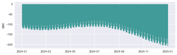
… which can be multiplied with the offtake in the following way, to increase the offtake with a varying percentage, that ranges from +0% on Jan 01 to +75% on Dec. 31:
[15]:
more_offtake = offtake * (1 + increase)
more_offtake.plot();
Combining volume and price
We can also combine the offtake volume with a price, which gives us a price-and-volume portfolio line. We can use fixed values, like here:
[16]:
offtake * pf.Q_(11.0, "ctEur/kWh")
[16]:
PfLine object with price and volume information.
. Start: 2024-01-01 00:00:00 (incl)    . Timezone    : none
. End  : 2025-01-01 00:00:00 (excl)    . Start-of-day: 00:00:00
. Freq : <Day> (366 datapoints)
                                     w           q           p             r
                                    MW         MWh     Eur/MWh           Eur

2024-01-01 00:00:00             -109.5      -2 628      110.00      -289 042
2024-01-02 00:00:00             -117.4      -2 818      110.00      -309 961
2024-01-03 00:00:00             -119.4      -2 866      110.00      -315 245
2024-01-04 00:00:00             -116.8      -2 803      110.00      -308 300
2024-01-05 00:00:00             -119.5      -2 868      110.00      -315 511
2024-01-06 00:00:00             -110.8      -2 659      110.00      -292 440
2024-01-07 00:00:00             -100.9      -2 422      110.00      -266 384
2024-01-08 00:00:00             -113.4      -2 721      110.00      -299 346
2024-01-09 00:00:00             -117.5      -2 821      110.00      -310 308
2024-01-10 00:00:00             -119.1      -2 858      110.00      -314 336
..                                  ..          ..          ..            ..
2024-12-23 00:00:00             -109.5      -2 628      110.00      -289 036
2024-12-24 00:00:00             -117.4      -2 817      110.00      -309 903
2024-12-25 00:00:00             -115.7      -2 777      110.00      -305 507
2024-12-26 00:00:00             -116.8      -2 803      110.00      -308 292
2024-12-27 00:00:00             -117.7      -2 825      110.00      -310 737
2024-12-28 00:00:00             -111.3      -2 672      110.00      -293 934
2024-12-29 00:00:00              -98.0      -2 352      110.00      -258 742
2024-12-30 00:00:00             -111.0      -2 664      110.00      -293 081
2024-12-31 00:00:00             -119.6      -2 870      110.00      -315 665
… or timeseries or other PfLine instances, like here:
[17]:
valued_offtake = offtake * prices # multiplying two PfLines
The resulting portfolio lines can again be resampled:
[18]:
valued_offtake.asfreq("QS")
[18]:
PfLine object with price and volume information.
. Start: 2024-01-01 00:00:00 (incl)    . Timezone    : none
. End  : 2025-01-01 00:00:00 (excl)    . Start-of-day: 00:00:00
. Freq : <QuarterBegin: startingMonth=1> (4 datapoints)
                                     w           q           p             r
                                    MW         MWh     Eur/MWh           Eur

2024-01-01 00:00:00             -110.0    -240 325      121.14   -29 111 995
2024-04-01 00:00:00              -85.4    -186 608       83.12   -15 509 925
2024-07-01 00:00:00              -78.5    -173 366       79.27   -13 743 550
2024-10-01 00:00:00             -103.2    -227 849      118.09   -26 907 440
Note that, even though prices and valued_offtake use the same price values at the daily resolution, the prices at quarterly resolution are slightly different. This is not an error: the values in prices are simply averaged (or actually, weighted with the duration of each timestamp, but those are uniform), whereas the values in valued_offtake are weighted with the energy in each timestamp.
This tutorial is continued in part 2.