PfState¶

A “portfolio state” (PfState) object stores the timeseries that relate to a portfolio at a certain moment in time. It stores information about the offtake in the portfolio; how much volume has currently been sourced and at what price; how much volume is consequently still unsourced and what is its current market price; what is the current best-guess for the procurement price of the portfolio (i.e., combining sourced and unsourced volumes to satisfy offtake), etc.

This page discusses their most important properties, and how to use them.

It is assumed that you are familiar with the PfLine class (link), and if you prefer a tutorial, see here.

Initialisation ¶

The state of a portfolio has 3 components, which are all specified with portfolio lines:

the offtake volume (volume-only portfolio line)
the price of the unsourced volume (price-only portfolio line)
the sourced volume (price-and-volume portfolio line)

If no volume has been sourced yet, it can be omitted.

With the .from_series() class method, initialisation is also possible from a set of pandas.Series, which are then internally converted into portfolio lines.

Both initialisation methods are shown here:

import portfolyo as pf, pandas as pd
index = pd.date_range('2024', freq='MS', periods=3)
w = pd.Series([-100, -250, -100], index, dtype='pint[MW]')
p = pd.Series([20, 22, 18], index, dtype='pint[Eur/MWh]')

# initialise from pflines
volume = pf.PfLine({'w': w})
prices = pf.PfLine({'p': p})
pfs = pf.PfState(volume, prices)

# initialise from series gives same object
pfs2 = pf.PfState.from_series(wo = w, pu = p) # same as pfs

# let's have a look at this portfolio state
pfs

PfState object.
. Start: 2024-01-01 00:00:00 (incl)    . Timezone    : none  
. End  : 2024-04-01 00:00:00 (excl)    . Start-of-day: 00:00:00  
. Freq : <MonthBegin> (3 datapoints)
                                                w           q           p             r
                                               MW         MWh     Eur/MWh           Eur
──────── offtake
           2024-01-01 00:00:00             -100.0     -74 400
           2024-02-01 00:00:00             -250.0    -174 000
           2024-03-01 00:00:00             -100.0     -74 400
─●────── pnl_cost
 │         2024-01-01 00:00:00              100.0      74 400       20.00     1 488 000
 │         2024-02-01 00:00:00              250.0     174 000       22.00     3 828 000
 │         2024-03-01 00:00:00              100.0      74 400       18.00     1 339 200
 ├────── sourced
 │         2024-01-01 00:00:00                0.0           0                         0
 │         2024-02-01 00:00:00                0.0           0                         0
 │         2024-03-01 00:00:00                0.0           0                         0
 └────── unsourced
           2024-01-01 00:00:00              100.0      74 400       20.00     1 488 000
           2024-02-01 00:00:00              250.0     174 000       22.00     3 828 000
           2024-03-01 00:00:00              100.0      74 400       18.00     1 339 200

Note that in this portfolio, no sourcing has yet taken place.

Unsourced price ¶

One of the parameters of the initialisation is the unsouncedprice, which needs a little bit of explanation. It is the price that we expect to pay (/receive) for the volume that the portfolio is currently short (/long). This is intimately connected to the market prices, but they are not necessarily equal.

If the portfolio state has the same frequency as the spot market on which any remaining open volume is eventually settled, the unsourcedprice can be set to the price-forward curve. It does not depend on the particulars of the portfolio we are considering – completely unhedged or nearly fully hedged; with its offtake predominantly during the day, during the night, during the week or during the weekend.

If the portfolio state is aggregated, e.g. to monthly values, we need to supply as unsourcedprice the average value of the price-forward curve in eath month weighted with the unsourced volume. This obviously does depend on the particulars of the portfolio. When comparing two portfolios with identical monthly offtake volumes and identical sourced volumes, the monthly unsourced price will be higher for the portfolio that has its offtake predominantly in the peak hours, compared to the other portfolio which has it mainly in the offpeak hours.

Warning

Some operations have as a consequence that the unsourced volume is changed, e.g., because they change the offtake or sourced volume. In this case, it is implicitly assumed that the original unsourced prices apply also to the updated unsourced volume. As explained, this assumption is not necessarily valid if the portfolio state is aggregated. A UserWarning is shown to alert the user to this possibility.

For this reason, it is often best/easiest to initialise portfolio states at the shorter time resolution: it allows us to always use the same unsourcedprice timeseries for each. If another frequency is wanted, we can leave the correct resampling (including the weighting) to the .asfreq() method, see the the section on resampling.

If the portfolio state includes past delivery periods, we must include sensible prices also for their unsourced volumes. Usually, the volumes and their financial impact are small, and we could use the spot prices to value them. In many circumstances, a different price, e.g. imbalance prices, is more applicable. If the portfolio state spans both past and future deliveries, the unsourced price timeseries also consists of a past and future section, likely having a distinct source.

Sign conventions ¶

The following conventions are used:

Volume that leaves the portfolio (e.g. due to offtake) is negative, volume that enters it (e.g. due to sourcing) is positive.
- Offtake should therefore be negative;
- Sourcing should be positive in the aggregate, though individual sourcing components can be negative, e.g. when selling long volumes on the spot market.
- In graphs, offtake and sourcing are often plotted on the same graph, or side-by-side. In that case the offtake is presented with positive values to facilitate the comparison.
Prices are positive when the buyer of a good pays money to the seller. This is the case in almost all market circumstances.
The result of the conventions above is that money that enters the portfolio is negative, and money that leaves it is positive. In general: monetary values can be seen as “costs”, with negative values being income.

Accessing data ¶

Several portfolio lines can be accessed as properties of a PfState object.

The portfolio lines used/created in the initialisation of the object:

.offtakevolume: volume-only portfolio line with offtake volume.
.sourced: price-and-volume portfolio line with volume that has currently been sourced.
.unsourcedprice: price-only portfolio line with the prices at which to value the volume that must still be procured to fully hedge the offtake profile.

And derived from these:

.unsourced: price-and-volume portfolio line. The prices are the unsourced prices; the volumes are those that are still unsourced, as calculated from the offtake volume and sourced volume.

# continuation from previous code example
pfs.unsourced

PfLine object with complete information.
. Start: 2024-01-01 00:00:00 (incl)    . Timezone    : none  
. End  : 2024-04-01 00:00:00 (excl)    . Start-of-day: 00:00:00  
. Freq : <MonthBegin> (3 datapoints)
                                     w           q           p             r
                                    MW         MWh     Eur/MWh           Eur

2024-01-01 00:00:00              100.0      74 400       20.00     1 488 000
2024-02-01 00:00:00              250.0     174 000       22.00     3 828 000
2024-03-01 00:00:00              100.0      74 400       18.00     1 339 200

.netposition: the same as unsourced, but with a reversed sign for the volume and revenue series. It shows the open positions in a way that is familiar for many portfolio managers, with negative volumes indicating short positions that must still be bought.
.sourcedfraction, .unsourcedfraction: pandas timeseries with the fraction of the offtake that has been (un)sourced. These two timeseries add up to 100% for each timestamp. In the example above, no sourcing has taken place, and so they are a uniform 0 and 1, respectively.
.pnl_cost: nested price-and-volume portfolio line, with children “sourced” and “unsourced” equal to the portfolio lines described above. This is one of the more important properties, as it shows the best estimate for the procurement price for each timestamp. In this case, this equals the unsourced price, as all offtake is unsourced.

# continuation from previous code example
pfs.pnl_cost

PfLine object with complete information.
. Start: 2024-01-01 00:00:00 (incl)    . Timezone    : none  
. End  : 2024-04-01 00:00:00 (excl)    . Start-of-day: 00:00:00  
. Freq : <MonthBegin> (3 datapoints)
. Children: 'sourced' (complete), 'unsourced' (complete)
                                     w           q           p             r
                                    MW         MWh     Eur/MWh           Eur

2024-01-01 00:00:00              100.0      74 400       20.00     1 488 000
2024-02-01 00:00:00              250.0     174 000       22.00     3 828 000
2024-03-01 00:00:00              100.0      74 400       18.00     1 339 200

See the tutorial for a more insightful example.

Plotting / Excel / Clipboard ¶

The .plot(), .to_excel() and .to_clipboard() methods exist similarly to on portfolio lines.

Plotting¶

# continuation from previous code example
pfs.plot()

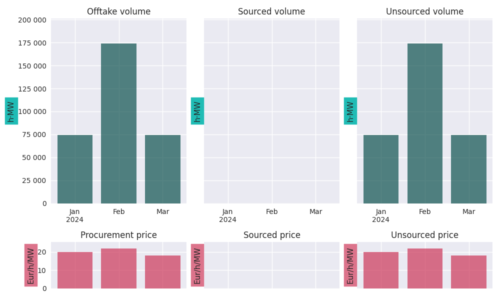
See the tutorial for an example with sourcing.

Excel and clipboard¶

Often, further data analyses are done in Excel. If you have a Workbook open, the easiest way is to copy the entire portfolio state data to the clipboard with the .to_clipboard() method. From there, it can be pasted onto a worksheet.

Alternatively, the data can be saved as an Excel workbook with the .to_excel() method.

# continuation from previous code example
pfs.to_clipboard()
pfs.to_excel("portfolio_state.xlsx")

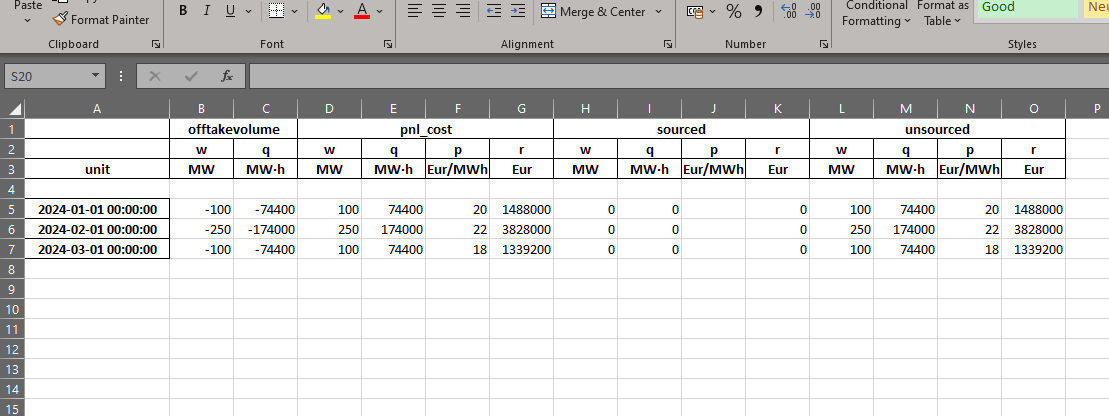
Of course, if only a part of the portfolio state is needed, we can also access the wanted portfolio line and copy/save only that, e.g. with pfs.sourced.to_clipboard().

Resampling ¶

As with portfolio lines, portfolio states can be resampled to a new frequency with the .asfreq() method. We usually downsample, e.g. from hourly to yearly values.

# continuation from previous code example
pfs.asfreq('QS')

PfState object.
. Start: 2024-01-01 00:00:00 (incl)    . Timezone    : none  
. End  : 2024-04-01 00:00:00 (excl)    . Start-of-day: 00:00:00  
. Freq : <QuarterBegin: startingMonth=1> (1 datapoints)
                                                w           q           p             r
                                               MW         MWh     Eur/MWh           Eur
──────── offtake
           2024-01-01 00:00:00             -147.8    -322 800
─●────── pnl_cost
 │         2024-01-01 00:00:00              147.8     322 800       20.62     6 655 200
 ├────── sourced
 │         2024-01-01 00:00:00                0.0           0                         0
 └────── unsourced
           2024-01-01 00:00:00              147.8     322 800       20.62     6 655 200

Notice how, for the unsourced volume, the prices are weighted with the energy in each month get the new price, just as is done with the sourced volume. Again, see the tutorial for a more elaborate example.

Arithmatic ¶

The following arithmetic operations are defined for portfolio states:

	Operation possible
`-PfState` (negation)	✅
`PfState ± PfState`	✅
`PfState * float`	✅
`PfState / float`	✅

Remarks:

The result of each of the operations above is another portfolio state.
The most common operation is to add or subtract portfolio states. In this case the individual components - offtake volume, sourced and unsourced volumes and revenues - are added/subtracted (according to the rules descibed in the relevant section on arithmatic with portfolio lines) and used to create the resulting portfolio state.
Negation is defined in such a way that it is consistent with pfs1 - pfs2 == pfs1 + -pfs2. It is identical to negating the portfolio lines for the offtake volume and sourced price-and-volume.
Multiplying with a factor means that the individual components are scaled. Specifically: the volumes (offtake, sourced, unsourced) are multiplied with the factor, while keeping the prices the same. This way, it is consistent with 2 * pfs == pfs + pfs.
Division by a factor is multiplying with its reciprocal, i.e., pfs / 2 == pfs * (1/2).
The multiplication or division factors do not have to be single values; we can also use a timeseries, in which case the multiplication/division are done on a per-timestamp basis.

Set portfolio lines ¶

To replace part of a portfolio state, we can use the .set_offtakevolume(), .set_unsourcedprice(), and .set_sourced() methods. These accept PfLine instances, and return a new portfolio state with the selected information replaced. Instead of setting the sourced price-and-volume, we can also add to the existing sourcing with the .add_sourced() method.

Note that, when changing the sourced or offtake volume, the warning in the section on unsourced prices applies.

Mark-to-Market ¶

If we want to know the market value of only the sourced volumes, we can use the .mtm_of_sourced() method, which calculates the surplus value of the sourcing contracts at current market prices. It uses the unsourced prices for this, so here too, the warning in the section on unsourced prices (above) applies.

Hedging ¶

The unsourced volume can be hedged with standard products - month, quarter, or year blocks. (See the section on heding in the documentation on portfolio lines). The .hedge_of_unsourced() method returns the portfolio line of the volumes and prices of this hedge; the .source_unsourced() method returns what the portfolio state would be, if this volume was actually added to the currently sourced volume.

Examples of this are shown in the tutorial.

API ¶

class portfolyo.PfState(offtakevolume: PfLine, unsourcedprice: PfLine, sourced: PfLine | None = None)¶

Class to hold timeseries information of an energy portfolio, at a specific moment.

Parameters:

offtakevolume (PfLine (volume-only))
unsourcedprice (PfLine (price-only))
sourced (PfLine (price-and-volume), optional) – If not specified, assume no sourcing has taken place.
offtakevolume. (All PfLines are trimmed to the length of the)

Notes

Sign conventions: - Volumes (q, w): >0 if volume flows into the portfolio. - Revenues (r): >0 if money flows out of the portfolio. Consequently, income is negative. - Prices (p): normally positive.

offtakevolume¶

Offtake. Volumes are <=0 for all timestamps (see ‘Notes’ above).

Type:: volume-only PfLine

sourced¶

Procurement. Volumes (and normally, revenues) are >=0 for all timestamps (see ‘Notes’ above).

Type:: price-and-volume PfLine

unsourced¶

Procurement/trade that is still necessary until delivery. Volumes (and normally, revenues) are >0 if more volume must be bought, <0 if volume must be sold for a given timestamp (see ‘Notes’ above). NB: if volume for a timestamp is 0, its price is undefined (NaN) - to get the market prices in this portfolio, use the property .unsourcedprice instead.

Type:: price-and-volume PfLine

unsourcedprice¶

Prices of the unsourced volume.

Type:: price-only PfLine

netposition¶

Net portfolio positions. Convenience property for users with a “traders’ view”. Does not follow sign conventions (see ‘Notes’ above); volumes are <0 if portfolio is short and >0 if long. Identical to .unsourced, but with sign change for volumes and revenues (but not prices).

Type:: price-and-volume PfLine

pnl_cost¶

The expected costs needed to source the offtake volume; the sum of the sourced and unsourced positions.

Type:: price-and-volume PfLine

asfreq(freq: str = 'MS') → PfState¶

Resample the Portfolio to a new frequency.

Parameters:: freq (str, optional) – The frequency at which to resample. ‘YS’ for year, ‘QS’ for quarter, ‘MS’ (default) for month, ‘D for day’, ‘h’ for hour, ‘15min’ for quarterhour.
Returns:: Resampled at wanted frequency.
Return type:: PfState

dataframe(cols: Iterable[str] | None = None, *args, has_units: bool = True, **kwargs) → DataFrame¶

DataFrame for portfolio state in default units.

Parameters:

cols (str, optional (default: all that are available)) – The columns (w, q, p, r) to include in the dataframe.
has_units (bool, optional (default: True)) –
- If True, return dataframe with pint units. (The unit can be extracted as a column level with .pint.dequantify()).
- If False, return dataframe with float values.

Return type:

pd.DataFrame

Create Portfolio instance from timeseries.

Parameters:

prices (unsourced) – pu [Eur/MWh]
volume (offtake) – qo [MWh] wo [MW]
revenue (sourced volume and) – (qs [MWh] or ws [MW]) rs [Eur] ps [Eur/MWh] If no volume has been sourced, all 4 sourced timeseries may be None.

Return type:

PfState

hedge_of_unsourced(how: str = 'val', peak_fn: Callable[[DatetimeIndex], Series] | None = None, freq: str = 'MS') → PfLine¶

Hedge the unsourced volume, at unsourced prices in the portfolio.

Parameters:

how (str, optional (Default: 'val')) – Hedge-constraint. ‘vol’ for volumetric hedge, ‘val’ for value hedge.
peak_fn (PeakFunction, optional (default: None)) – To hedge with peak and offpeak products: function that returns boolean Series indicating if timestamps in index lie in peak period. If None, hedge with base products.
freq ({'D' (days), 'MS' (months, default), 'QS' (quarters), 'YS' (years)}) – Frequency of hedging products. E.g. ‘QS’ to hedge with quarter products.

See also

PfLine.hedge_with, portfolyo.create_peakfn, portfolyo.germanpower_peakfn

Returns:: Hedge (volumes and prices) of unsourced volume.
Return type:: PfLine

property index: DatetimeIndex¶: Left timestamp of time period corresponding to each data row.

property loc: _LocIndexer¶: Create a new instance with a subset of the rows (selection by row label(s) or a boolean array.)

mtm_of_sourced() → PfLine¶: Mark-to-Market value of sourced volume.

plot(children: bool = False) → plt.Figure¶

Plot the portfolio state.

Parameters:: None
Returns:: The figure object to which the series was plotted.
Return type:: plt.Figure

print(num_of_ts: int = 5, color: bool = True) → None¶

Treeview of the portfolio state.

Parameters:

num_of_ts (int, optional (default: 5)) – How many timestamps to show for each PfLine.
color (bool, optional (default: True)) – Make tree structure clearer by including colors. May not work on all output devices.

Return type:

None

property slice: _SliceIndexer¶: Create a new instance with a subset of the rows. Different from loc since performs slicing with right-open interval.

source_unsourced(how: str = 'val', peak_fn: Callable[[DatetimeIndex], Series] | None = None, freq: str = 'MS') → PfState¶

Simulate PfState if unsourced volume is hedged and sourced at market prices.

Parameters:

how (str, optional (Default: 'val')) – Hedge-constraint. ‘vol’ for volumetric hedge, ‘val’ for value hedge.
peak_fn (PeakFunction, optional (default: None)) – To hedge with peak and offpeak products: function that returns boolean Series indicating if timestamps in index lie in peak period. If None, hedge with base products.
freq ({'D' (days), 'MS' (months, default), 'QS' (quarters), 'YS' (years)}) – Frequency of hedging products. E.g. ‘QS’ to hedge with quarter products.

See also

PfState.hedge_of_unsourced

Returns:: which is fully hedged at time scales of freq or longer.
Return type:: PfState

to_clipboard(*, excel: bool = True, sep: str | None = None, **kwargs) → None¶

Copy object to the system clipboard.

Write a text representation of object to the system clipboard. This can be pasted into Excel, for example.

Parameters:

excel (bool, default True) –
Produce output in a csv format for easy pasting into excel.
- True, use the provided separator for csv pasting.
- False, write a string representation of the object to the clipboard.
sep (str, default '\t') – Field delimiter.
**kwargs – These parameters will be passed to DataFrame.to_csv.

See also

DataFrame.to_csv: Write a DataFrame to a comma-separated values (csv) file.
read_clipboard: Read text from clipboard and pass to read_csv.

Notes

Requirements for your platform.

Linux : xclip, or xsel (with PyQt4 modules)

Windows : none

macOS : none

This method uses the processes developed for the package pyperclip. A solution to render any output string format is given in the examples.

Examples

Copy the contents of a DataFrame to the clipboard.

>>> df = pd.DataFrame([[1, 2, 3], [4, 5, 6]], columns=['A', 'B', 'C'])

>>> df.to_clipboard(sep=',')  
... # Wrote the following to the system clipboard:
... # ,A,B,C
... # 0,1,2,3
... # 1,4,5,6

We can omit the index by passing the keyword index and setting it to false.

>>> df.to_clipboard(sep=',', index=False)  
... # Wrote the following to the system clipboard:
... # A,B,C
... # 1,2,3
... # 4,5,6

Using the original pyperclip package for any string output format.

import pyperclip
html = df.style.to_html()
pyperclip.copy(html)

to_excel(excel_writer: FilePath | WriteExcelBuffer | ExcelWriter, *, sheet_name: str = 'Sheet1', na_rep: str = '', float_format: str | None = None, columns: Sequence[Hashable] | None = None, header: Sequence[Hashable] | bool_t = True, index: bool_t = True, index_label: IndexLabel | None = None, startrow: int = 0, startcol: int = 0, engine: Literal['openpyxl', 'xlsxwriter'] | None = None, merge_cells: bool_t = True, inf_rep: str = 'inf', freeze_panes: tuple[int, int] | None = None, storage_options: StorageOptions | None = None, engine_kwargs: dict[str, Any] | None = None) → None¶

Write object to an Excel sheet.

To write a single object to an Excel .xlsx file it is only necessary to specify a target file name. To write to multiple sheets it is necessary to create an ExcelWriter object with a target file name, and specify a sheet in the file to write to.

Multiple sheets may be written to by specifying unique sheet_name. With all data written to the file it is necessary to save the changes. Note that creating an ExcelWriter object with a file name that already exists will result in the contents of the existing file being erased.

Parameters:

excel_writer (path-like, file-like, or ExcelWriter object) – File path or existing ExcelWriter.
sheet_name (str, default 'Sheet1') – Name of sheet which will contain DataFrame.
na_rep (str, default '') – Missing data representation.
float_format (str, optional) – Format string for floating point numbers. For example float_format="%.2f" will format 0.1234 to 0.12.
columns (sequence or list of str, optional) – Columns to write.
header (bool or list of str, default True) – Write out the column names. If a list of string is given it is assumed to be aliases for the column names.
index (bool, default True) – Write row names (index).
index_label (str or sequence, optional) – Column label for index column(s) if desired. If not specified, and header and index are True, then the index names are used. A sequence should be given if the DataFrame uses MultiIndex.
startrow (int, default 0) – Upper left cell row to dump data frame.
startcol (int, default 0) – Upper left cell column to dump data frame.
engine (str, optional) – Write engine to use, ‘openpyxl’ or ‘xlsxwriter’. You can also set this via the options io.excel.xlsx.writer or io.excel.xlsm.writer.
merge_cells (bool, default True) – Write MultiIndex and Hierarchical Rows as merged cells.
inf_rep (str, default 'inf') – Representation for infinity (there is no native representation for infinity in Excel).
freeze_panes (tuple of int (length 2), optional) – Specifies the one-based bottommost row and rightmost column that is to be frozen.
storage_options (dict, optional) –
Extra options that make sense for a particular storage connection, e.g. host, port, username, password, etc. For HTTP(S) URLs the key-value pairs are forwarded to urllib.request.Request as header options. For other URLs (e.g. starting with “s3://”, and “gcs://”) the key-value pairs are forwarded to fsspec.open. Please see fsspec and urllib for more details, and for more examples on storage options refer here.

Added in version 1.2.0.
engine_kwargs (dict, optional) – Arbitrary keyword arguments passed to excel engine.

See also

to_csv: Write DataFrame to a comma-separated values (csv) file.
ExcelWriter: Class for writing DataFrame objects into excel sheets.
read_excel: Read an Excel file into a pandas DataFrame.
read_csv: Read a comma-separated values (csv) file into DataFrame.
io.formats.style.Styler.to_excel: Add styles to Excel sheet.

Notes

For compatibility with to_csv(), to_excel serializes lists and dicts to strings before writing.

Once a workbook has been saved it is not possible to write further data without rewriting the whole workbook.

Examples

Create, write to and save a workbook:

>>> df1 = pd.DataFrame([['a', 'b'], ['c', 'd']],
...                    index=['row 1', 'row 2'],
...                    columns=['col 1', 'col 2'])
>>> df1.to_excel("output.xlsx")  

To specify the sheet name:

>>> df1.to_excel("output.xlsx",
...              sheet_name='Sheet_name_1')  

If you wish to write to more than one sheet in the workbook, it is necessary to specify an ExcelWriter object:

>>> df2 = df1.copy()
>>> with pd.ExcelWriter('output.xlsx') as writer:  
...     df1.to_excel(writer, sheet_name='Sheet_name_1')
...     df2.to_excel(writer, sheet_name='Sheet_name_2')

ExcelWriter can also be used to append to an existing Excel file:

>>> with pd.ExcelWriter('output.xlsx',
...                     mode='a') as writer:  
...     df1.to_excel(writer, sheet_name='Sheet_name_3')

To set the library that is used to write the Excel file, you can pass the engine keyword (the default engine is automatically chosen depending on the file extension):

>>> df1.to_excel('output1.xlsx', engine='xlsxwriter')  